Creating Security Decision Trees With Graphviz

In the recently published “Security Chaos Engineering” e-book, one of the chapters I wrote covers attacker math and the power of decision trees to guide more pragmatic threat modelling. This post will walk through creating the example decision tree from the e-book using Graphviz and a .DOT file.¹

Using this as a reference, you can extrapolate this process into a pattern to inform saner security prioritization during the design phase of the product lifecycle. I won’t cover how to populate your own decision tree in this post since that is already covered in the e-book, which is immediately available at your fingertips for the delectable price of free.

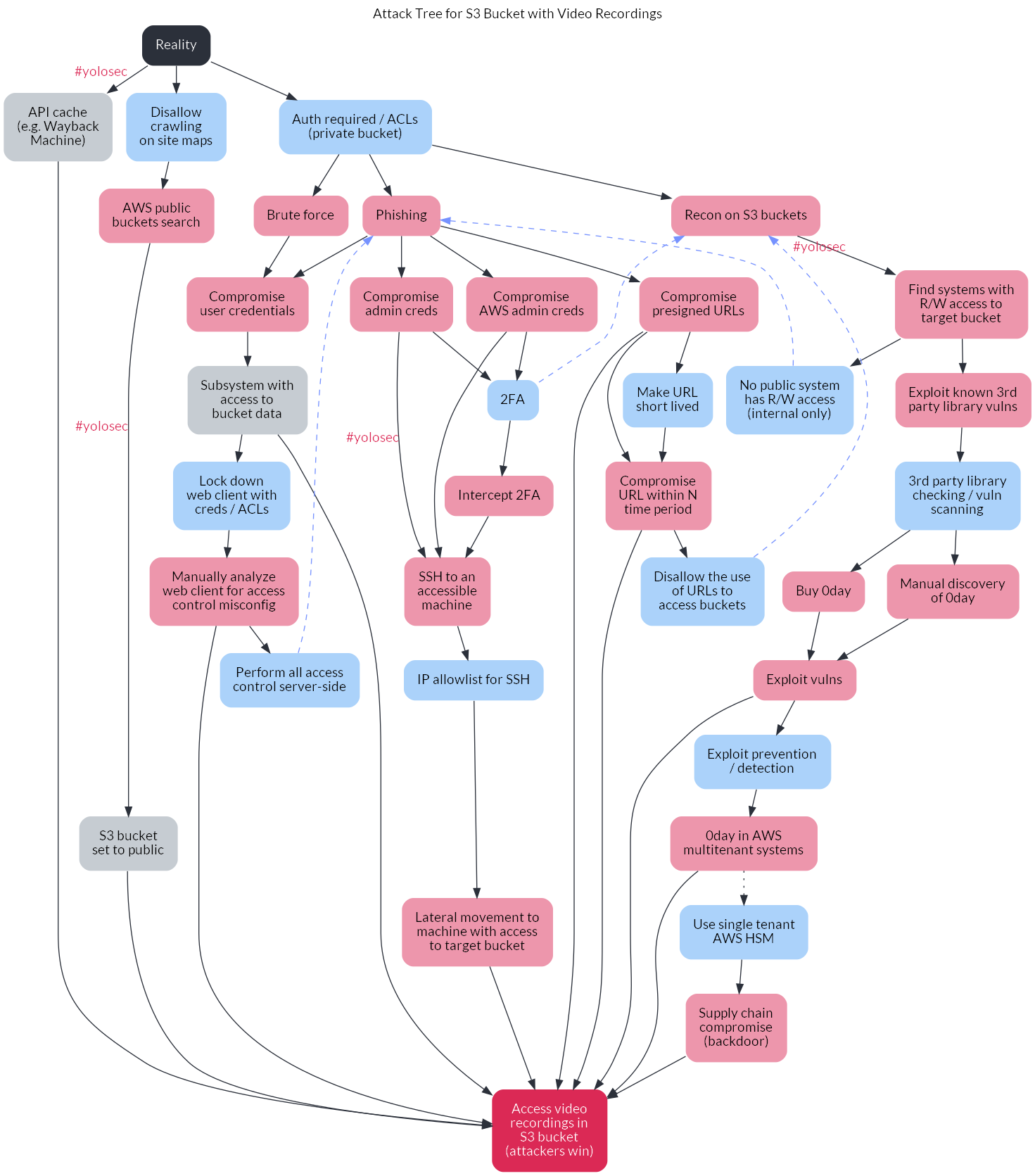
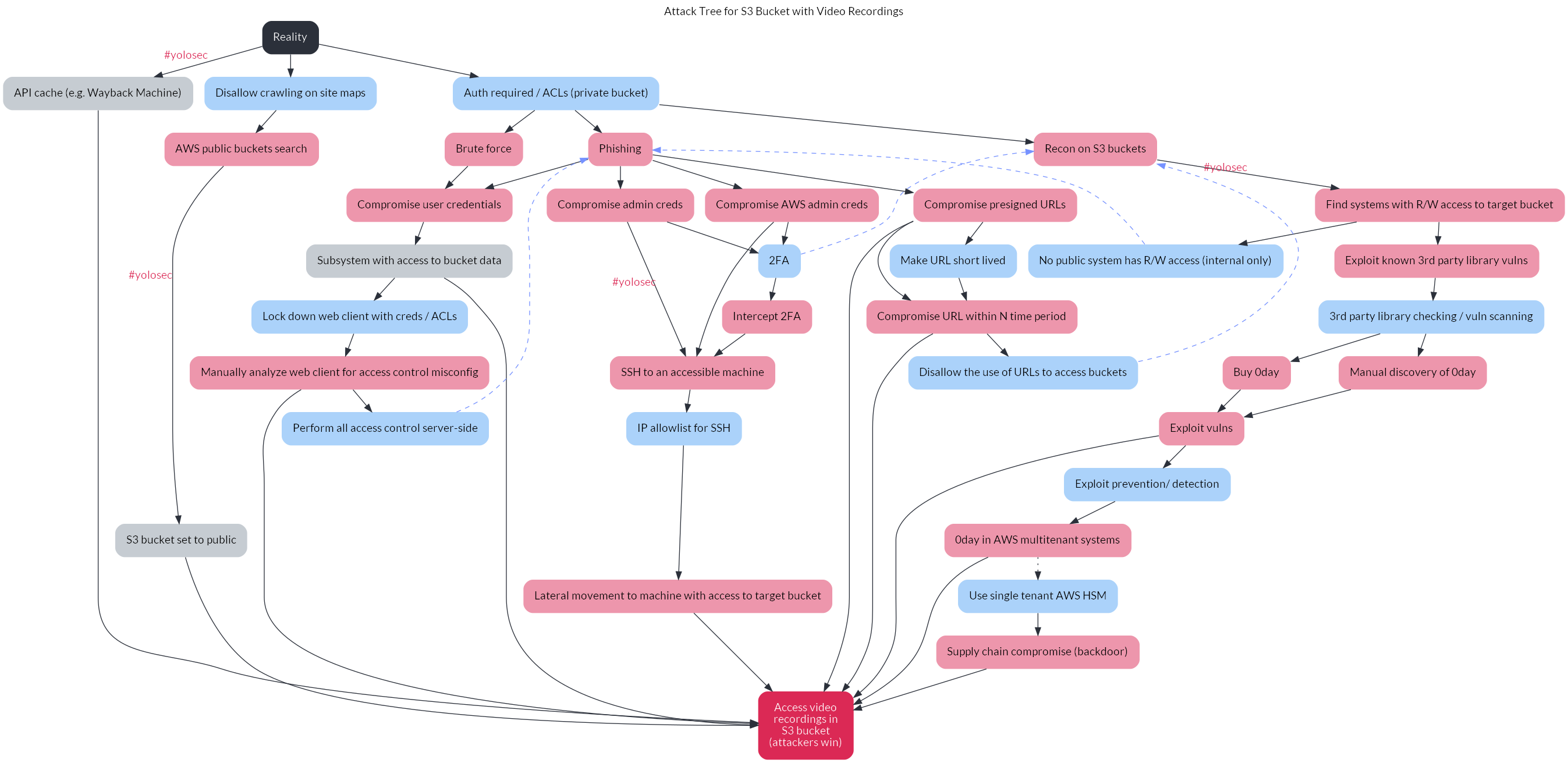
As an apéritif, here’s the end result towards which we’ll be building:

A brief intro on Graphviz

As the name suggests, Graphviz is a graph visualization tool. It is open source, which was especially compelling as I tried out various graphing tools for the decision tree use case because I am a ho for not spending money.

Graphviz takes descriptions of graphs in text form and converts them into a visual (like an image or PDF). I found that the default styling options for Graphviz can quickly look like a hybrid of the infamous defense charts or the “graphic design is my passion” meme. However, these style deficiencies are balanced by the ease of editing the relationships represented in the graph – an issue I previously found tedious when using GUI-based tools.

The textual descriptions of the graph are written using the DOT language (and thereby saved as a .DOT file). I personally found it quite intuitive, though, as always, your mileage may vary.

Building the decision tree

For those of you who haven’t read the report yet (reminder: it’s free), let’s set some background context on this example.

Organizations often store important content in cloud storage buckets. In this example, our imaginary organization wants to store customer video recordings in an S3 bucket. As the product and engineering teams think through the design of this project, they want to avoid bad things happening to the project that could cost money (whether via downtime or compliance fines) or time (which is also money)².

The (rather obvious) way attackers win is by successfully accessing the video recordings in the S3 bucket. Thus, the decision tree shows the potential paths attackers can take, including attacker actions performed in response to defensive actions or mitigations, to reach the goal of accessing that S3 bucket.

The branches of the tree are oriented from the lowest cost paths to attackers (on the left) to the most expensive attacker paths (on the right). The lowest cost path for attackers is generally the one with zero defensive mitigations in place, what I affectionately call “yolosec.” The highest cost path for attackers usually involves finding and exploiting zero day vulnerabilities or performing upstream supply chain attacks³.

If you want to understand more about the decision tree architecture, I entreat you yet again to download the Security Chaos Engineering report.

Step 1 - Defining the basic nodes

The most basic security decision tree will have two common states: Reality (the starting node from which all others descend)⁴ and Attackers Win (the ending node reflecting attackers accomplishing their goal).⁵

All the branches on the tree – reflecting different cost paths – will end up connecting the Reality and Attackers Win nodes in some fashion.

Let’s define these states in a .dot file (I named mine sce-tree.dot). We’re going to be using a digraph, which is short for “directed graph.” Directed graphs show one-way relationships, whereas undirected graphs show symmetrical relationships.

Your initial code thus looks like:

digraph {
	reality
	attack_win 
}

reality and attack_win are our first two nodes. We don’t have any attributes for them yet (styling will come later), so it looks pretty plain.

In this example, we know that the asset we’re threat modelling is the S3 bucket with video recordings, so we can apply a label to the attack_win node saying as much. That way, when the graph is visualized, the node will read as “Access video recordings in S3 bucket” rather than “attack_win”.

To create this label, we add brackets after the relevant node to contain the attribute label="Access video recordings in S3 bucket". There are a bunch of attributes you can assign to nodes (like styling), but we’ll cover more of those later.

For now, the foundation for our threat model decision tree looks like this:

digraph {
	reality [ label="Reality" ]
	attack_win [ label="Access video recordings in S3 bucket" ]
}

Step 2 - Creating the first attack node

The first branch in the decision tree should represent the lowest cost attack path. In the example from the SCE report, the branch barely involves an attack – it assumes #yolosec, representing a reality in which you’ve allowed crawling on your sitemap, enabling cache APIs (like the Wayback machine) to create caches of the bucket’s contents.

This means our first attack node is actually more of a state of being. The only attacker action is to access this API cache, for which we will create a new node:

digraph {
	// base nodes
	reality [ label="Reality" ]
	attack_win [ label="Access video recordings in S3 bucket" ]

	// attack nodes
	attack_1 [ label="API cache (e.g. Wayback Machine)" ]
}

You have a few options for how you want to define the nodes in your decision tree. Above, I defined the node as attack_1, since I personally find it easier to keep track of attack (and defense) actions sequentially. However, you can also define the nodes more explicitly, such as api_cache, like so:

	// attack nodes
	api_cache [ label="API cache (e.g. via Wayback machine)" ]
	toothbrush_0day [ label="0day in your electric toothbrush" ]
	planet_hax [ label="Hack the planet!"]
}

You can also use letters, like A, B, C, etc., but I personally find it crude and harder to follow relative to the more descriptive options as the tree gets more complex.

You’ll also note I’ve commented the heading // attack nodes. I find it easier to separate out attack vs. defense nodes, especially when it comes to styling (as we’ll see first in step 6). Another option is to organize your nodes within the .dot file by branch, such as:

digraph {
	// base nodes
	reality [ label="Reality" ]
	attack_win [ label="Access video recordings in S3 bucket" ]

	// branch 1
	attack_1 [ label="API cache (e.g. via Wayback machine)" ]
	defense_1 [ label="#yolosec" ]

	// branch 2
	attack_2 [ label="0day in your electric toothbrush" ]
	defense_2 [ label="roll over and play dead" ]
}

Whatever your preference, just make sure you’re consistent as you continue to build out the tree. Also note that Graphviz does not warn you if there are duplicate nodes, so choose whichever organization option will minimize the probability of you creating duplicates.

Step 3 - Creating the first branch edges

Because I’m impatient and maybe you are, too, let’s work towards visualizing this first branch so we can see something tangible from our efforts thus far. This means we need to create the edges for the first branch.

Edges are the connectors between nodes. Because our decision trees are causal diagrams, we’ll be using the -> edge (i.e. arrowhead edge) to represent a directional flow of action.

In the case of this first branch, we start from the reality node, which connects to the #yolosec state of an API cache existing, which leads to attackers successfully accessing the bucket data (and thus winning). In our .dot file, these edges will be defined like this:

digraph {
	// base nodes
	reality [ label="Reality" ]
	attack_win [ label="Access video recordings in S3 bucket" ]

	// attack nodes
	attack_1 [ label="API cache (e.g. Wayback Machine)" ]

	// branch 1 edges
	reality -> attack_1
	attack_1 -> attack_win
}

If you want to highlight what a snafu the API cache is, you can even add a “#yolosec” label (via xlabel=) to the edge:

reality -> attack_1 [ xlabel="#yolosec" ]
attack_1 -> attack_win

Step 4 - Visualizing the first branch

Now that we have the necessary nodes and edges for our first branch, let’s visualize it! Spoiler alert: without any styling, it’s not going to look too pretty.

I find a PDF to be the most digestible format for decision trees, since it allows better zooming and panning than an image (like a .png). However, for obvious reasons, I’ll be using .png’s to illustrate the results of each command throughout this post.

To create a PDF of our decision tree thus far, we can use the command: dot -Tpdf sce-tree.dot -o attack-tree.pdf

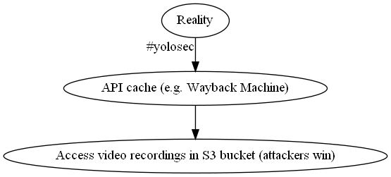
That is super hideous! But we successfully visualized that a reality in which an API cache of our video recordings is available leads to attackers winning with minimal effort (with the #yolosec tag for extra flair).

Step 5 - Filling out another branch

Now it’s time to add another branch. This will involve creating new attack nodes, defense nodes, and edges between them.

Because we learned our lesson on the dangers of #yolosec, we know that we should implement the mitigation of disallowing crawling on our site maps. This will be our first defense node:

digraph {
	// base nodes
	reality [ label="Reality" ]
	attack_win [ label="Access video recordings in S3 bucket (attackers win)" ]

	// attack nodes
	attack_1 [ label="API cache (e.g. Wayback Machine)" ]

	// defense nodes
	defense_1 [ label="Disallow crawling on site maps" ]

	// branch 1 edges
	reality -> attack_1 [ xlabel="#yolosec" ]
	attack_1 -> attack_win
}

As discussed in the SCE report, we next need to think about how an attacker will respond to our mitigations (what is known as “belief prompting”). The easiest thing an attacker can do next, if an API cache isn’t available, is searching public buckets to see if the target data is accessible. This will be our second node among our attack nodes:

// attack nodes
attack_1 [ label="API cache (e.g. Wayback Machine)" ]
attack_2 [ label="AWS public buckets search" ]

We will again assume #yolosec – that our S3 bucket is set to public and thus accessible via search. This will be our third attack node:

// attack nodes
attack_1 [ label="API cache (e.g. Wayback Machine)" ]
attack_2 [ label="AWS public buckets search" ]
attack_3 [ label="S3 bucket set to public" ]

With all our nodes defined for the second branch, we now need to connect them via edges:

digraph {
	// base nodes
	reality [ label="Reality" ]
	attack_win [ label="Access video recordings in S3 bucket (attackers win)" ]

	// attack nodes
	attack_1 [ label="API cache (e.g. Wayback Machine)" ]
	attack_2 [ label="AWS public buckets search" ]
	attack_3 [ label="S3 bucket set to public" ]

	// defense nodes
	defense_1 [ label="Disallow crawling on site maps" ]

	// branch 1 edges
	reality -> attack_1 [ xlabel="#yolosec" ]
	attack_1 -> attack_win

	// branch 2 edges
	reality -> defense_1
	defense_1 -> attack_2
	attack_2 -> attack_3 [ xlabel="#yolosec" ]
	attack_3 -> attack_win
}

We can overwrite our prior file with this new branch by running the same command again: dot -Tpdf sce-tree.dot -o attack-tree.pdf

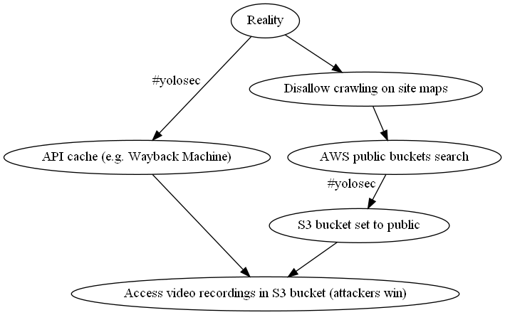
We can now see how the attackers must change their actions when a mitigation is place. However, it is still ugly af.

Step 6 - Differentiating between attack & defense nodes

While we’ll take care of the hideousness later when we apply real styling, you can probably already tell just from two branches that differentiating between attack and defense nodes can get confusing quickly – especially as we keep adding nodes.

Luckily, Graphviz allows you to define styling specific to a list of nodes. Given we already have separate lists of attack and defense nodes, we can add different colors for each by adding the color attribute at the beginning of the list using node [ color="#hexgoeshere" ]. This will start as an outline color for now but result in a fill color once we apply more styling in step 8.

Let’s start by applying a pale raspberry color to our attack actions:

// attack nodes
node [ color="#ED96AC" ]
attack_1 [ label="API cache (e.g. Wayback Machine)" ]
attack_2 [ label="AWS public buckets search" ]
attack_3 [ label="S3 bucket set to public" ]

Then, we can add a pale blue color for our defense actions (matching the common red team vs. blue team parlance):

// defense nodes
node [ color="#ABD2FA" ]
defense_1 [ label="Disallow crawling on site maps" ]

Let’s see how this looks by running our command again:

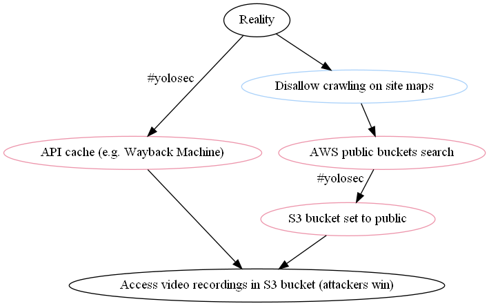
Astute readers may quibble that the existence of an API cache and the public bucket setting aren’t really attacker actions. Graphviz allows you to style nodes individually, too – so we can apply a grey color to the attack nodes that moreso reflect conditions that facilitate attack success:

// attack nodes
node [ color="#ED96AC" ]
attack_1 [ label="API cache (e.g. Wayback Machine)" color="#C6CCD2" ]
attack_2 [ label="AWS public buckets search" ]
attack_3 [ label="S3 bucket set to public" color="#C6CCD2" ]

Finally, we can add some colors for our base nodes: a bold strawberry for our Attackers Win ;_; condition and a charcoal one for our Reality node:

reality [ label="Reality" color="#2B303A" ]
attack_win [ label="Access video recordings in S3 bucket (attackers win)" color="#DB2955" ]

When we run dot -Tpdf sce-tree.dot -o attack-tree.pdf again, we can now differentiate between the various nodes:

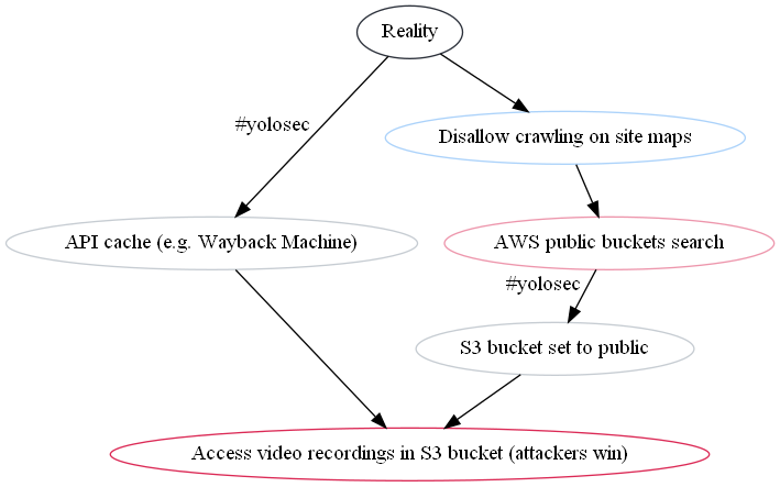
With this super basic styling set up for better readability as we build out the tree, let’s get to the next branches – many of which are more complicated.

Step 7 - Drawing the Owl

To shorten an already lengthy post, we will walk through the third branch but then add the rest of the nodes and edges roughly en masse so we can move onto the styling and ordering steps.

This is a bit of a “draw the owl” moment, but hopefully you can extrapolate from the fully fleshed example branches to the rest – connecting the .dots, as it were – using the complete decision tree in the report as a reference.

However, because I’m not totally heartless, I also created a GitHub repo containing the dot files and graph images for each of the branches so you can see the changes along the way.

Filling out the third branch

This branch starts with our final mitigation that directly descends from the reality branch. Learning our #yolosec lesson yet again, we see that making the S3 bucket private and having some sort of access control on it is a sensible mitigation. This is reflected in our second node among the defense nodes:

// defense nodes
node [ color="#ABD2FA" ]
defense_1 [ label="Disallow crawling on site maps" ]
defense_2 [ label="Auth required / ACLs (private bucket)" ]  

What will attackers do in response? Well, they’ll probably try to brute force their way in (usually the lower-cost option) or try to phish credentials of users with access to the bucket. They could also try to perform reconnaissance on our organization’s S3 buckets, but that is a more expensive option which we will reflect on a later branch.

For now, we add the former two options to our list of attack nodes:

// attack nodes
node [ color="#ED96AC" ]
attack_1 [ label="API cache (e.g. Wayback Machine)" color="#C6CCD2" ]
attack_2 [ label="AWS public buckets search" ]
attack_3 [ label="S3 bucket set to public" color="#C6CCD2" ]
attack_4 [ label="Brute force" ]
attack_5 [ label="Phishing" ]

If brute forcing is successful, then attackers can compromise user credentials – and the same with phishing. Logging in with those credentials (“creds”), the attacker can find a subsystem with access to the target bucket data, leading to an attacker win.

However, we can potentially mitigate subsystem access -> bucket access by locking down our web client with creds or access control lists (ACLs). In response, the attacker will need to manually analyze the web client for some sort of access control misconfiguration so they can still access the target S3 bucket – and thus still win.

We can mitigate that attacker response, too, by ensuring we perform all access control server-side. With these easier options thwarted, attackers will need to go back to the phishing drawing board and aim for more privileged credentials (which you can see on branch 4).

Putting this flow of attacker action -> defender response -> attacker response together, we now have these attack and defense nodes:

// attack nodes
node [ color="#ED96AC" ]
attack_1 [ label="API cache (e.g. Wayback Machine)" color="#C6CCD2" ]
attack_2 [ label="AWS public buckets search" ]
attack_3 [ label="S3 bucket set to public" color="#C6CCD2" ]
attack_4 [ label="Brute force" ]
attack_5 [ label="Phishing" ]
attack_6 [ label="Compromise user credentials" ]
attack_7 [ label="Subsystem with access to bucket data" color="#C6CCD2" ]
attack_8 [ label="Manually analyze web client for access control misconfig" ]

// defense nodes
node [ color="#ABD2FA" ]
defense_1 [ label="Disallow crawling on site maps" ]
defense_2 [ label="Auth required / ACLs (private bucket)" ]
defense_3 [ label="Lock down web client with creds / ACLs" ]
defense_4 [ label="Perform all access control server-side" ]

Now we need to connect them to reflect the “If This, Then That”-style logic of the attacker / defender game at hand. There are a few decision forks here depending on whether or not there is a mitigation. I find it useful to comment // potential mitigation at those forks for clarity, as shown here:

// branch 3 edges
reality -> defense_2
defense_2 -> attack_4
defense_2 -> attack_5
attack_4 -> attack_6
attack_5 -> attack_6
attack_6 -> attack_7
attack_7 -> attack_win
// potential mitigation path
attack_7 -> defense_3
defense_3 -> attack_8
attack_8 -> attack_win
// potential mitigation path
attack_8 -> defense_4 
defense_4 -> attack_5 [ style="dashed" color="#7692FF" ]

To reflect the fact that our last mitigation (performing access control server-side) sends attackers back up the tree to try a more expensive branch, I’ve styled the last edge as a dashed line with a periwinkle color.

Running our output command again, we can see the three branches together:

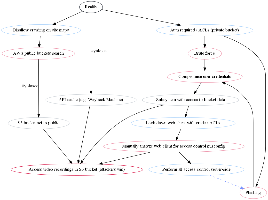
Well… it’s technically correct, but organized in a weird way that makes it pretty tricky to follow. Since we have five more branches to add, it doesn’t make sense for us to tweak the ordering yet – that will be covered in step 9.

Adding branches 4 - 7

To keep this post moving, I beseech you to review the .dot files and graph outputs in the GitHub repo for the rest of the branches through the last one (branch 8). There is also commentary within the .dot files for each of the branches skipped over here for your perusal.

Your .dot file ahead of the final branch should look like this:

digraph {
	// base nodes
	reality [ label="Reality" color="#2B303A" ]
	attack_win [ label="Access video recordings in S3 bucket (attackers win)" color="#DB2955" ]

  	// attack nodes
  	node [ color="#ED96AC" ]
	attack_1 [ label="API cache (e.g. Wayback Machine)" color="#C6CCD2" ]
	attack_2 [ label="AWS public buckets search" ]
	attack_3 [ label="S3 bucket set to public" color="#C6CCD2" ]
	attack_4 [ label="Brute force" ]
	attack_5 [ label="Phishing" ]
	attack_6 [ label="Compromise user credentials" ]
	attack_7 [ label="Subsystem with access to bucket data" color="#C6CCD2" ]
	attack_8 [ label="Manually analyze web client for access control misconfig" ]
	attack_9 [ label="Compromise admin creds" ]
	attack_10 [ label="Intercept 2FA" ]
	attack_11 [ label="SSH to an accessible machine" ]
	attack_12 [ label="Lateral movement to machine with access to target bucket" ]
	attack_13 [ label="Compromise AWS admin creds" ]
	attack_14 [ label="Compromise presigned URLs" ]
	attack_15 [ label="Compromise URL within N time period" ]
	attack_16 [ label="Recon on S3 buckets" ]
	attack_17 [ label="Find systems with R/W access to target bucket" ]
	attack_18 [ label="Exploit known 3rd party library vulns" ]

	// defense nodes
	node [ color="#ABD2FA" ]
	defense_1 [ label="Disallow crawling on site maps" ]
	defense_2 [ label="Auth required / ACLs (private bucket)" ]
	defense_3 [ label="Lock down web client with creds / ACLs" ]
	defense_4 [ label="Perform all access control server-side" ]
	defense_5 [ label="2FA" ]
	defense_6 [ label="IP allowlist for SSH" ]
	defense_7 [ label="Make URL short lived" ]
	defense_8 [ label="Disallow the use of URLs to access buckets" ]
	defense_9 [ label="No public system has R/W access (internal only)" ]
	defense_10 [ label="3rd party library checking / vuln scanning" ]

	// branch 1 edges
	reality -> attack_1 [ xlabel="#yolosec" fontcolor="#DB2955" ]
	attack_1 -> attack_win	

	// branch 2 edges
	reality -> defense_1
	defense_1 -> attack_2
	attack_2 -> attack_3 [ xlabel="#yolosec" fontcolor="#DB2955" ]
	attack_3 -> attack_win

	// branch 3 edges
	reality -> defense_2
	defense_2 -> attack_4
	defense_2 -> attack_5
	attack_4 -> attack_6
	attack_5 -> attack_6
	attack_6 -> attack_7
	attack_7 -> attack_win
	// potential mitigation path
	attack_7 -> defense_3
	defense_3 -> attack_8
	attack_8 -> attack_win
	// potential mitigation path
	attack_8 -> defense_4 
	defense_4 -> attack_5 [ style="dashed" color="#7692FF" ]
	
	// branch 4 edges
	attack_5 -> attack_9
	attack_9 -> attack_11 [ xlabel="#yolosec" fontcolor="#DB2955" ]
	// potential mitigation path
	attack_9 -> defense_5 
	defense_5 -> attack_10 
	attack_10 -> attack_11
	// potential mitigation path
	attack_11 -> defense_6 
	defense_6 -> attack_12 
	attack_12 -> attack_win

	// branch 5 edges
	attack_5 -> attack_13
	attack_13 -> attack_11
	attack_13 -> defense_5

	// branch 6 edges
	attack_5 -> attack_14
	attack_14 -> attack_win
	attack_14 -> attack_15
	// potential mitigation path
	attack_14 -> defense_7 
	defense_7 -> attack_15 
	attack_15 -> attack_win
	// potential mitigation path
	attack_15 -> defense_8 

	// branch 7 edges
	defense_2 -> attack_16
	defense_5 -> attack_16 [ style="dashed" color="#7692FF" ]
	defense_8 -> attack_16 [ style="dashed" color="#7692FF" ]
	attack_16 -> attack_17 [ xlabel="#yolosec" fontcolor="#DB2955" ]
	// potential mitigation path
	attack_17 -> defense_9 
	defense_9 -> attack_5 [ style="dashed" color="#7692FF" ]
	attack_17 -> attack_18
	// potential mitigation path
	attack_18 -> defense_10

}

Adding the last branch (branch 8)

We’re now on the hardest branch for attackers, the one requiring zero-day (“0day”) exploits or supply chain backdoors. These are expensive, whether in money or time, so attackers will generally use them as a last resort or if the return on investment (ROI) is more favorable – such as when those actions enable the ability to gain access to a bunch of organizations in one fell swoop, avoiding the need to compromise them individually.

Our last mitigation from the seventh branch was vulnerability (“vuln”) scanning, (ideally) eliminating the option for attackers to exploit a known vuln. Thus, attackers will either need to buy 0day or discover and develop 0day themselves. A potential mitigation to 0day exploits is, somewhat obviously, exploit detection and prevention.

Assuming this mitigation actually works⁶, attackers will be forced to try 0day affecting AWS multitenant systems. In response, defenders could adopt a single tenant AWS hardware security module (HSM) model, which would then force attackers to plant a backdoor in a component in AWS’s supply chain.

For the purposes of illustration, I’ve assumed that the organization creating this decision tree / threat model does not currently employ AWS HSMs. Therefore, the edge leading to that defense node is styled as a dotted line.

This final branch results in the following new nodes and edges:

attack_19 [ label="Manual discovery of 0day" ]
attack_20 [ label="Buy 0day" ]
attack_21 [ label="Exploit vulns" ]
attack_22 [ label="0day in AWS multitenant systems" ]
attack_23 [ label="Supply chain compromise (backdoor)" ]

defense_11 [ label="Exploit prevention/ detection" ]
defense_12 [ label="Use single tenant AWS HSM" ]

// branch 8 edges
defense_10 -> attack_19
defense_10 -> attack_20
attack_19 -> attack_21
attack_20 -> attack_21
attack_21 -> attack_win
// potential mitigation path
attack_21 -> defense_11 
defense_11 -> attack_22 
attack_22 -> attack_win 
// potential mitigation path
attack_22 -> defense_12 [ style="dotted" ]
defense_12 -> attack_23 
attack_23 -> attack_win

With all our nodes and edges now in place, our graph looks like this:

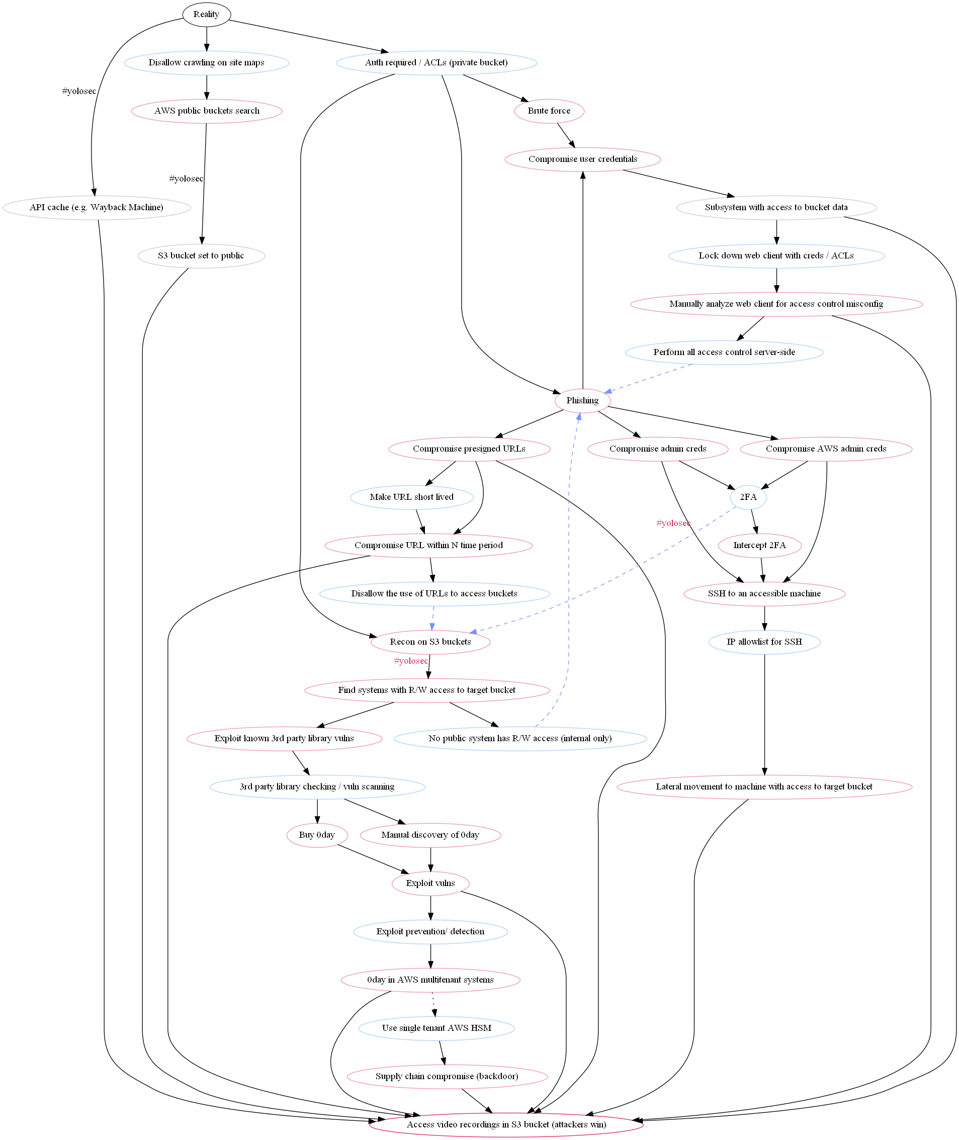
It is very ugly and difficult to follow. We should proceed to the next steps so that we do not have to stare at this monstrosity further.

Step 8 - Beautifying the graph

Before we tackle the fact that many of the nodes are out of intended order, we should try to make this all look less hideous. Graphviz allows for some limited styling options, which, to be honest, I mostly figured out through guess and check given how sparse I found the docs to be.

Node styling

Let’s start by making the nodes less Word 95-era design. I personally chose to replace the outlines with a fill, using the same colors as before.

You can set global node design by inserting node [ * ] at the beginning of your .dot file. To get rid of the outlines, add the shape attribute with the value plaintext and add the style attribute with the value filled, rounded (I possess a fondness for rounded edges):

digraph {
	// Base Styling
	node [ shape="plaintext" style="filled, rounded" ]

Because nodes are now filled with the previously-defined colors, we also need to lighten the font color for the reality and attack_win nodes; I chose white:

// base nodes
reality [ label="Reality" fillcolor="#2B303A" fontcolor="#ffffff" ]
attack_win [ label="Access video recordings in S3 bucket (attackers win)"
fillcolor="#DB2955" fontcolor="#ffffff" ]

Also, who uses Times New Roman anymore? Apparently Graphviz does, since it’s the default font. Let’s change the font to Lato:

// Base Styling
node [ shape="plaintext" style="filled, rounded" fontname="Lato"]

Finally, we can make the nodes a bit roomier by adding a slight margin around the text within:

// Base Styling
node [ shape="plaintext" style="filled, rounded" fontname="Lato" margin=0.2]

Our graph now looks like this with the new node styling:

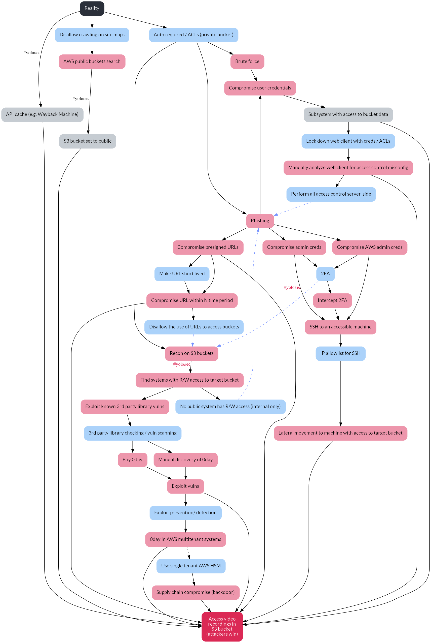
It’s already looking more modern! But we can do more.

Edge styling

We can make the edges prettier, too, by changing the #yolosec label font to Lato and by lightening the lines up slightly so they aren’t in stark black:

// Base Styling
node [ shape="plaintext" style="filled, rounded" fontname="Lato"]
edge [ fontname="Lato" color="#2B303A" ]

We can see the results of our slight changes here:

Graph styling

There’s a lot of whitespace in our graph right now, which arguably reduces navigability. Ideally, the graph should be a solidly readable size in the Page Width view in a PDF reader. So, let’s reduce some of the white space.

We can set styling for the whole graph by inserting it above the node [ * ] and edge [ * ] base styling we added above. Let’s start by reducing the horizontal distance between nodes via the nodesep attribute and the vertical distance via the ranksep attribute:

// Base Styling
nodesep="0.2";
ranksep="0.4";
node [ shape="plaintext" style="filled, rounded" fontname="Lato" margin=0.2]
edge [ fontname="Lato" color="#2B303A" ]

For this next styling option, I’m going to level with y’all: this combination resulted in the best visual outcomes after a lot of guess and check, but I’m still not 100% what they do. In any case, setting splines=true and overlap=false seems to generate the cleanest visualization:

// Base Styling
splines=true;
overlap=false;
nodesep="0.2";
ranksep="0.4";
node [ shape="plaintext" style="filled, rounded" fontname="Lato" margin=0.2]
edge [ fontname="Lato" color="#2B303A" ]

I also added in the attribute specifying the graph should be visualized from top to bottom, even though it’s the default (I am risk averse):

rankdir="TB";

Last, but certainly not least, I titled the graph using the label attribute and set the label location to the top with labelloc. With all of this incorporated, the base styling section in the .dot file now looks like this:

// Base Styling
rankdir="TB";
splines=true;
overlap=false;
nodesep="0.2";
ranksep="0.4";
label="Attack Tree for S3 Bucket with Video Recordings";
labelloc="t";
fontname="Lato";
node [ shape="plaintext" style="filled, rounded" margin=0.2 fontname="Lato" ]
edge [ fontname="Lato" color="#2B303A" ]

With the new styling complete, our graph looks much more visually appealing:

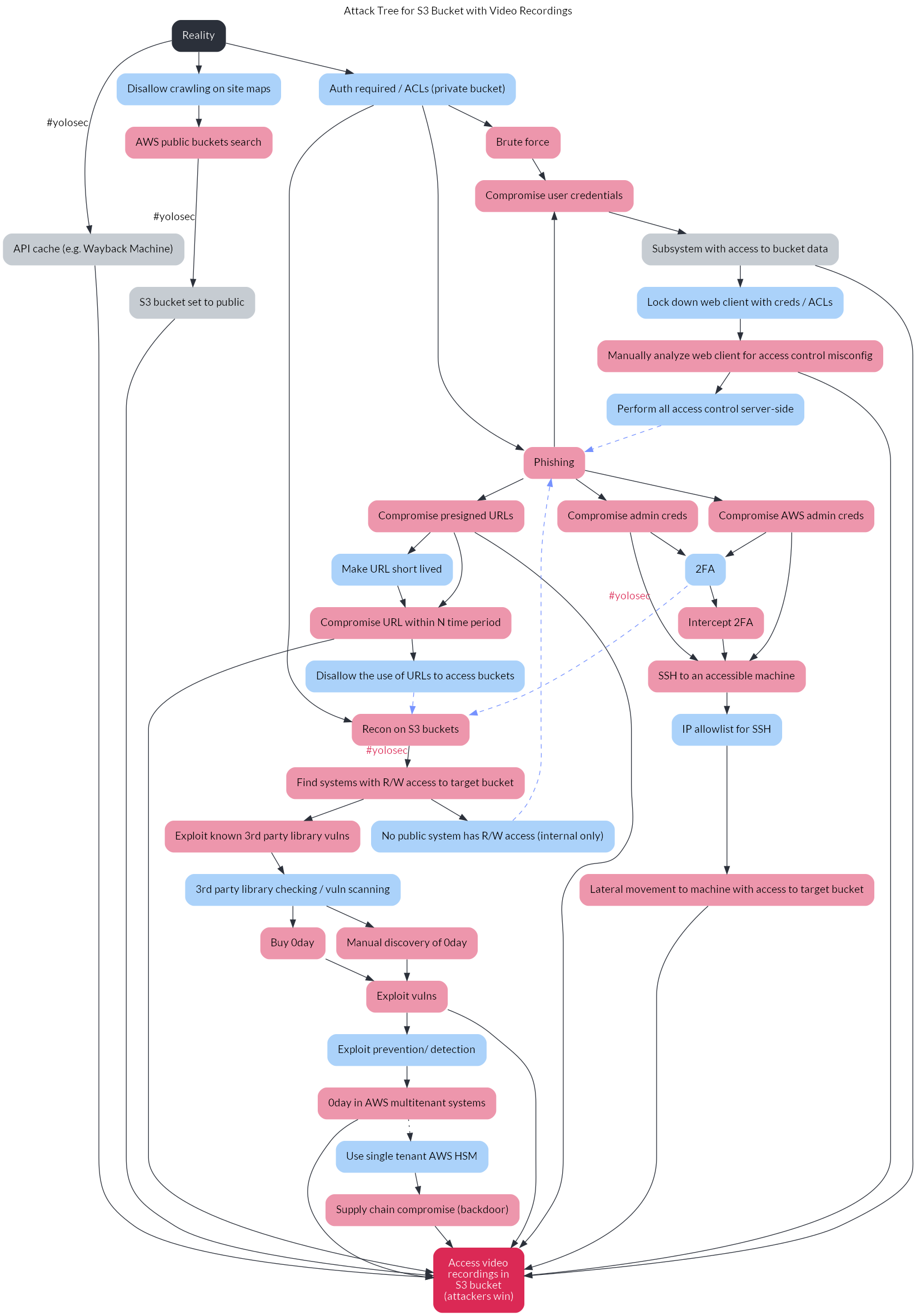
However, it’s still a little confusing due to the errant default node placement by Graphviz. We’ll fix this in the next step.

Step 9 - Fixing the ordering

One of the benefits of the decision tree is to visualize a threat model in order of easiest / lowest cost attacker path to hardest / highest cost attacker path (generally from left to right). By default, Graphviz does not respect the order in which we’ve written our nodes and edges, necessitating some fixes.

I approached this necessary re-ordering by creating a cluster for each group of nodes that should be equal in hierarchy. In Graphviz, a cluster is encoded as a subgraph, which can be used for a variety of purposes beyond the aesthetic ordering one in this post.

The three clusters in our tree diagram are:

• The initial nodes after the reality node: the API cache, disallowing crawling on site maps, and private buckets
• The attack nodes after auth is required: brute force, phishing, and recon on s3 buckets
• The subsequent attack nodes after phishing: compromise user creds, admin creds, AWS admin creds, or pre-signed URLs

We can encode these clusters as subgraphs with the attribute rank=same (to weight the nodes equally in the hierarchy) along with the list of relevant nodes in the cluster:

// Subgraphs / Clusters
subgraph initialstates {
	rank=same;
	attack_1;
	defense_1;
	defense_2;
}

subgraph authrequired {
	rank=same;
	attack_4;
	attack_5;
	attack_16;
}

subgraph phishcluster {
	rank=same;
	attack_6;
	attack_9;
	attack_13;
	attack_14;
} 

I would like to spare y’all the vexation I experienced when Graphviz didn’t respect the order in which I listed the nodes within a cluster. For instance, instead of showing attack_4 as the leftmost node in the authrequired cluster and attack_16 as the rightmost, Graphviz seemed to prefer to use a methodology reflected by ¯\_(ツ)_/¯.

What seems to fix this ordering issue is creating invisible edges that enforce the left to right ordering. For our graph, the fix is specifically found in enforcing the correct order in the phishcluster subgraph:

attack_6 -> attack_9 -> attack_13 -> attack_14 [ style="invis" ]

Aren’t computers great? In any case, our graph now accurately visualizes the ordering of our decision tree:

Step 10 - Tweaking the design

There are other tweaks we can make to make this graph (and the .dot file itself!) more digestible.

I chose to add line breaks for particularly long node labels, such as label="API cache\n(e.g. Wayback\nMachine)", and definitely recommend it for your own tree. I also added in more comments to the .dot file so that someone else reading it could better understand what is going on.

With these last tweaks, this is how our final .dot file looks:⁷

digraph {
	// Base Styling
	rankdir="TB";
	splines=true;
	overlap=false;
	nodesep="0.2";
	ranksep="0.4";
	label="Attack Tree for S3 Bucket with Video Recordings";
	labelloc="t";
	fontname="Lato";
	node [ shape="plaintext" style="filled, rounded" fontname="Lato" margin=0.2 ]
	edge [ fontname="Lato" color="#2B303A" ]

	// List of Nodes

	// base nodes
	reality [ label="Reality" fillcolor="#2B303A" fontcolor="#ffffff" ]
	attack_win [ label="Access video\nrecordings in\nS3 bucket\n(attackers win)" fillcolor="#DB2955" fontcolor="#ffffff" ]

  	// attack nodes
  	node [ color="#ED96AC" ]
	attack_1 [ label="API cache\n(e.g. Wayback\nMachine)" color="#C6CCD2" ]
	attack_2 [ label="AWS public\nbuckets search" ]
	attack_3 [ label="S3 bucket\nset to public" color="#C6CCD2" ]
	attack_4 [ label="Brute force" ]
	attack_5 [ label="Phishing" ]
	attack_6 [ label="Compromise\nuser credentials" ]
	attack_7 [ label="Subsystem with\naccess to\nbucket data" color="#C6CCD2" ]
	attack_8 [ label="Manually analyze\nweb client for access\ncontrol misconfig" ]
	attack_9 [ label="Compromise\nadmin creds" ]
	attack_10 [ label="Intercept 2FA" ]
	attack_11 [ label="SSH to an\naccessible\nmachine" ]
	attack_12 [ label="Lateral movement to\nmachine with access\nto target bucket" ]
	attack_13 [ label="Compromise\nAWS admin creds" ]
	attack_14 [ label="Compromise\npresigned URLs" ]
	attack_15 [ label="Compromise\nURL within N\ntime period" ]
	attack_16 [ label="Recon on S3 buckets" ]
	attack_17 [ label="Find systems with\nR/W access to\ntarget bucket" ]
	attack_18 [ label="Exploit known 3rd\nparty library vulns" ]
	attack_19 [ label="Manual discovery\nof 0day" ]
	attack_20 [ label="Buy 0day" ]
	attack_21 [ label="Exploit vulns" ]
	attack_22 [ label="0day in AWS\nmultitenant systems" ]
	attack_23 [ label="Supply chain\ncompromise\n(backdoor)" ]

	// defense nodes
	node [ color="#ABD2FA" ]
	defense_1 [ label="Disallow\ncrawling\non site maps" ]
	defense_2 [ label="Auth required / ACLs\n(private bucket)" ]
	defense_3 [ label="Lock down\nweb client with\ncreds / ACLs" ]
	defense_4 [ label="Perform all access\ncontrol server-side" ]
	defense_5 [ label="2FA" ]
	defense_6 [ label="IP allowlist for SSH" ]
	defense_7 [ label="Make URL\nshort lived" ]
	defense_8 [ label="Disallow the use\nof URLs to\naccess buckets" ]
	defense_9 [ label="No public system\nhas R/W access\n(internal only)" ]
	defense_10 [ label="3rd party library\nchecking / vuln\nscanning" ]
	defense_11 [ label="Exploit prevention\n/ detection" ]
	defense_12 [ label="Use single tenant\nAWS HSM" ]

	// List of Edges

	// branch 1 edges
	// this starts from the reality node and connects with the first "attack",
	// which is really just taking advantage of #yolosec (big oof)
	reality -> attack_1 [ xlabel="#yolosec" fontcolor="#DB2955" ]
	attack_1 -> attack_win	

	// branch 2 edges
	// this connects the reality node to the first mitigation, 
	// which helps avoid the #yolosec path from branch 1
	reality -> defense_1
	defense_1 -> attack_2
	attack_2 -> attack_3 [ xlabel="#yolosec" fontcolor="#DB2955" ]
	attack_3 -> attack_win

	// branch 3 edges
	// this connects the reality node to another mitigation,
	// which helps avoid the #yolosec path from branch 2
	reality -> defense_2
	defense_2 -> attack_4
	defense_2 -> attack_5
	attack_4 -> attack_6
	attack_5 -> attack_6
	attack_6 -> attack_7
	attack_7 -> attack_win
	// potential mitigation path
	attack_7 -> defense_3
	defense_3 -> attack_8
	attack_8 -> attack_win
	// potential mitigation path
	attack_8 -> defense_4 
	defense_4 -> attack_5 [ style="dashed" color="#7692FF" ]
	
	// branch 4 edges
	// this starts from the last mitigation loop vs. the reality node
	attack_5 -> attack_9
	attack_9 -> attack_11 [ xlabel="#yolosec" fontcolor="#DB2955" ]
	// potential mitigation path
	attack_9 -> defense_5 
	defense_5 -> attack_10 
	attack_10 -> attack_11
	// potential mitigation path
	attack_11 -> defense_6 
	defense_6 -> attack_12 
	attack_12 -> attack_win

	// branch 5 edges
	// this also represents a branch from the prior mitigation loop
	// but it is more difficult than branch 4, hence comes after
	// the new attack step allows attackers to skip some steps on branch 4
	// so it links back to branch 4, whose edges are already defined
	attack_5 -> attack_13
	attack_13 -> attack_11
	attack_13 -> defense_5

	// branch 6 edges
	// depending on the mitigations, the initial node allows for different outcomes
	// this also represents a branch from the prior mitigation loop
	// it is more difficult than branch 4 and branch 5, hence comes after
	attack_5 -> attack_14
	attack_14 -> attack_win
	attack_14 -> attack_15
	// potential mitigation path
	attack_14 -> defense_7 
	defense_7 -> attack_15 
	attack_15 -> attack_win
	// potential mitigation path
	attack_15 -> defense_8 

	// branch 7 edges
	// a new loop is born!
	// the first edges tie prior mitigations to the new attack step
	defense_2 -> attack_16
	defense_5 -> attack_16 [ style="dashed" color="#7692FF" ]
	defense_8 -> attack_16 [ style="dashed" color="#7692FF" ]
	attack_16 -> attack_17 [ xlabel="#yolosec" fontcolor="#DB2955" ]
	// potential mitigation path
	attack_17 -> defense_9 
	defense_9 -> attack_5 [ style="dashed" color="#7692FF" ]
	attack_17 -> attack_18
	// potential mitigation path
	attack_18 -> defense_10

	// branch 8 edges
	// we've reached the last path!
	// this is the most expensive one for attackers.
	// these attacks are definitely uncommon...
	// ...because attackers will be cheap / lazy if they can be.
	// these edges start from the last mitigation from branch 7
	defense_10 -> attack_19
	defense_10 -> attack_20
	attack_19 -> attack_21
	attack_20 -> attack_21
	attack_21 -> attack_win
	// potential mitigation path
	attack_21 -> defense_11 
	defense_11 -> attack_22 
	attack_22 -> attack_win 
	// potential mitigation path
	// for the purposes of illustration, this path represents a mitigation
	// that isn't actually implemented yet -- hence a dotted edge
	attack_22 -> defense_12 [ style="dotted" ]
	defense_12 -> attack_23 
	attack_23 -> attack_win

	// Subgraphs / Clusters

	// these clusters enforce the correct hierarchies
	subgraph initialstates {
    	rank=same;
    	attack_1;
    	defense_1;
    	defense_2;
  	}
	subgraph authrequired {
    	rank=same;
    	attack_4;
    	attack_5;
    	attack_16;
  	}
  	subgraph phishcluster {
    	rank=same;
    	attack_6;
    	attack_9;
    	attack_13;
    	attack_14;
    	rankdir=LR;
  	}
  	// these invisible edges are to enforce the correct left-to-right order 
  	// based on the level of attack difficulty
  	attack_6 -> attack_9 -> attack_13 -> attack_14 [ style="invis" ]
}

Conclusion

After these ten steps, we’ve successfully recreated the decision tree from the SCE report and optimized it for readability, too:

While it may feel daunting to create your first decision tree in this manner, the good news is you now have a base template with styling that you can use to threat model other critical assets.

If you try this out yourself or for your own organization, I welcome any and all feedback on how the .dot config or process itself can be improved. Security chaos engineering is a blossoming discipline bearing real potential to make infosec finally not suck, so we should help each other level up however we can.

---

Thank you shoutout to Team Bad <3